Because I’m quite short on my 52 posts this year, I’m stealing this from the lab blog (which I wrote!). But hey! First research paper published, jeez what a long process…
Highlights (tl;dr)
The overarching goal of our recent NeuroImage paper (PDF) is to make inferences about the brain’s synaptic/molecular-level processes using large-scale (very much non-molecular or microscopic) electrical recordings. In the following blog post, I will take you through the concept of excitation- inhibition (EI) balance, why it’s important to quantify, and how we go about doing so in the paper, which is the novel contribution. It’s aimed at a broad audience, so there are a lot of analogies and oversimplifications, and I refer you to the paper itself for the gory details. At the end, I reflect a little on the process and talk about the real (untold) story of how this paper came to be. **
A Tale of Two Forces
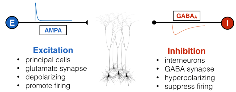
Inside all of our brains, there are two fundamental and opposing forces – no, not good and evil – excitation and inhibition. Excitatory input, well, “excites” a neuron, causing it to depolarize (become more positively charged internally) and fire off an action potential if enough excitatory inputs converge. This is the fundamental mechanism by which neurons communicate: shorts bursts of electrical impulses. Inhibitory inputs, on the other hand, do exactly the opposite: they hyperpolarize a neuron, making it less likely to fire an action potential. Not to be hyperbolic, but since before you were born these two forces were waging war with and balancing one another through embryonic development, infancy, childhood, adulthood, and till death. There are lots of molecular mechanisms for excitation and inhibition, but for the most part, “excitatory neurons” are responsible for sending excitation via a neurotransmitter called glutamate, and “inhibitory neurons” are responsible for inhibition via GABA.
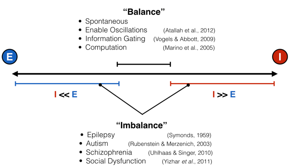
Like all great rivalries (think Batman and Joker, Celtics and Lakers), these two forces cannot exist without each other, but they also keep each other in check: too much excitation leads the brain to have run-away activity, such as what happens in seizure, while too much inhibition shuts everything down, as happens during sleep, anesthesia, or being drunk. This makes intuitive sense, and scientists have empirically validated this “excitation-inhibition balance” concept numerous times. This EI balance, as it’s called, is ubiquitous under normal conditions, and has been proposed to be crucial for neural computation, the routing of information in the brain, and many other processes. Furthermore, it’s been hypothesized, with some experimental evidence in animals, that an imbalance of excitation and inhibition is the cause (or result) of many neurological and psychiatric disorders, including epilepsy, schizophrenia, and autism, just to name a few.
Finding Balance
Given how important this intricate balance is, it is actually quite difficult to measure at any moment the ratio between excitatory and inhibitory inputs. I mentioned above that there is empirical evidence for balance and imbalance. However, in the vast majority of these cases, measurements are done by poking tiny electrodes into single neurons and, via a protocol called voltage clamping, scientists record within a single neuron how much excitatory and inhibitory input that neuron is receiving. Because the setup is so delicate, it’s often done in slices of brain tissue kept alive in a dish, or sometimes in a head-fixed, anesthetized mouse or rat – basically, in brain tissue that can’t move much, but not in humans. I mean, imagine doing this in the intact brain of a living human – yeah, I can’t either. And as far as I know, it’s never been done. This presents a pretty big conundrum: if we want to link a psychiatric disorder to an improper ratio between excitation and inhibition in the human brain directly, but we can’t actually measure that thing, how can we corroborate that EI (im)balance matters in the way we think it does?
Our Approach: Parsing Balance From “Background Noise”
This is exactly the problem we try to solve in our recent paper published in NeuroImage : how might one estimate the ratio between excitation and inhibition in a brain region without having to invasively record from within a brain cell (which is not something most people would like to happen to them)?
Well, recording inside a brain cell is hard, but recording outside brain cells – extracellularly – is a LOT easier. It’s still pretty invasive, depending on the technique, but much safer and more feasible in moving, living, behaving people. Of course, recording outside the brain cell is not the same as recording the inside – when we record electrical fluctuations in the space around neurons, rather from within or right next to a single neuron, we’re picking up the activity of thousands to millions of cells all mixed up together.
The first critical idea of our paper was that this aggregate signal – often referred to as the local field potential (LFP) – reflects excitatory and inhibitory inputs onto a large population of local cells, not just a single one. Therefore, we should be able to get a general estimate of balance by decoding this aggregate signal. The second piece of critical information was the realization that (for the most part) excitatory inputs are fast and inhibitory inputs are slow so that, even when they are mixed together from millions of different sources like in the LFP signal, we are still able to separate their effects: not in time, but in the frequency-domain (see our frequency domain tutorial).
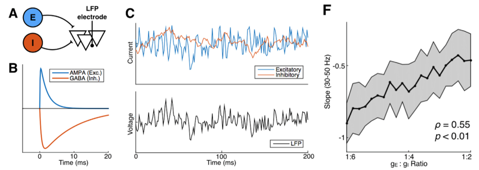 A: LFP model with excitatory and inhibitory inputs; B: the time course of E
and I inputs from a single action potential; C: simulated synaptic inputs
(blue and red) and LFP (black); F: LFP index of E:I ratio
A: LFP model with excitatory and inhibitory inputs; B: the time course of E
and I inputs from a single action potential; C: simulated synaptic inputs
(blue and red) and LFP (black); F: LFP index of E:I ratio
Combining Computational Modeling and Empirical (Open) Data
Pursuing this line of reasoning, we simulated populations of neurons in silico and looked at how their activity would generate a local field potential recording. What this means is that we can generate, in a computer simulation, different ratios of excitatory or inhibitory inputs into a brain region and see how that influences the simulated LFP. Through this computational model we found an index for the relative ratio between excitation and inhibition.
For those of you that are into frequency-domain analysis of neural signal, this index is the 1/f power law exponent of the LFP power spectrum. Let’s unpack that a bit. In the figure above (panel B) you can see that the excitatory electrical currents (blue) that contribute to the LFP shoot up in voltage really quickly—within a few thousands of a second—and then slowly decay back down to zero. In contrast, the inhibitory currents (red) also shoot up pretty quickly—but not as quickly—and then decay back to zero much more slowly than the excitatory inputs. When you add up thousands of these currents happening all at different times, the simulated voltage (panel C, black) looks to us humans a lot like noise. But through the mathematical magic of the Fourier transform, when we look at this same signal’s frequency representation, they’re clearly distinguishable!
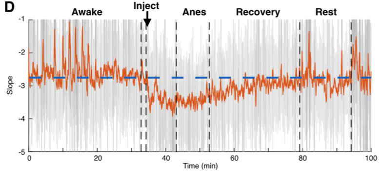
More technically, the idea is that the ratio between fast excitation and slow inhibition should be represented by the relative strength between high- frequency (rapidly fluctuating) and low-frequency (slowly fluctuating) signals. With this hypothesis in hand, we were able to make use of several publicly available databases of neural recordings to validate the predictions made by our computational models in a few different ways. One example from the paper: we were lucky enough to find a recording from macaque monkeys undergoing anesthesia, and the anesthetic agent, propofol, acts through amplifying inhibitory inputs in the brain at GABA synapses. Therefore, we predicted that when the monkey goes under, we should see a corresponding change in the power law exponent, and that’s exactly what we found! As you can see below, our EI index remains relatively stable during the awake state, then immediately shoots down toward an inhibition-greater-than-excitation regime during the anesthetized state before coming back to baseline after the anesthesia wears off.
Takeaways and Disclaimers
So to summarize, we were able to make predictions, borne out of observations from previous physiological experiments and our own computational modeling, and then validate these predictions using data from existing databases to draw a link between EI balance, which is a cellular-level process, and the local field potential, which is an aggregate circuit-level signal. Personally, I think that bridging the gap between these different levels of description in the brain is super interesting, and it’s one way for us to confirm our understanding of how the brain gives rise to cognition and behavior at multiple scales. Furthermore, we can now make use of the theoretical idea of EI balance in places where it was previously inaccessible, such as a human patients responding to treatments.
Before I wrap up, I just want to point out that this paper does not conclusively show that EI balance directly shifts the power law exponent – what we show is a suggestive correlation. Nor does the correlation hold under all circumstances. We had to make a lot of assumptions in our model and the data we found, such as the noise-like process by which we generated the model inputs. I’m not throwing this out here to inhibit the excitement (hah, hah), but rather to limit the scope of our claim, especially for a public-facing blog piece like this.
Rather, ours is the first step of an ongoing investigation, and although we will probably find evidence that corroborates and contradicts our findings later on, it’s important that anyone reading this and getting excited (hah) about it understands that we do not, and likely will not, have the last word on this. Ultimately, though, I believe we stumbled onto something pretty cool and we’ll definitely follow up on those assumptions one by one, and hopefully have more blog posts to come!
Some Personal Reflection
This project was my first real scientific research project in grad school, and it definitely created in me a lot of joy and excitement, as well as caused a fair amount of brooding. As a whole, I really enjoyed the process of building a computational model, even if it was quite simple, and using the predictions from that to inform further empirical investigations. As I mentioned, I think we really need to bridge the gap between molecular-level mechanisms in the brain and circuit/organism-level “neural markers”, and computational modeling work allows us to do that in situations where it would be intractable for many reasons. I certainly subscribe to the notion that combining theoretical/computational work with empirical data is an exciting and fruitful line of research, because it fills a space between two successful but largely non-overlapping subfields in neuroscience (though that trend is now changing).
Also, the fact that we were able to test our predictions on publicly available data was such a blessing, as we simply did not have the capacity, as a new lab, to do those in vitro and in vivo experiments ourselves. However, that meant combing through tons and tons of data where there might have been unlabeled or badly labeled information, only to reach the conclusion that the data is unusable for our purposes. There was some (a lot) of headbanging due to this, but ultimately, we found useful (FREE!) data and I’m very grateful for the people that made them available: CRCNS and Buzsaki Lab, Neurotycho and Fujii Lab, as well as many friends and collaborators that donated data for us to test different routes. To support this open-access endeavor, all code used to produce the analysis and figures are on our lab GitHub, found here.
The Untold Story
One last note, for those of you that find the process of scientific discovery interesting: in this blog post, I tried to write the story as a lay-friendly CliffsNotes version of the paper, starting with the importance of EI balance and the motivation to find an accessible index of it in the LFP, then outlining how we went about solving that problem. That’s the scientific story, and while not false, it’s not chronological.
The actual story began with Brad’s 2015 paper showing that aging is associated with 1/f changes. That was actually what first interested me back when I started in 2014 – this seemingly ubiquitous phenomenon (1/f scaling) in neural data. After digging a bit to find various accounts for how 1/f observations arise in nature, we decided to just simulate the LFP ourselves and see what happens. Turns out, the 1/f naturally falls out of the temporal profile of synaptic currents, which both have exponential rise and decay.
Our model contained what I thought to be the bare minimum: excitatory and inhibitory currents. At that point, I didn’t have a clue about what EI balance was and what it has been linked to. I think I was twiddling parameters one day, and realized that changing the relative weight of E and I inputs will cause the 1/f exponent (or slope) to change because of their different time constants. Then, like any modern-day graduate student, I Googled to see if this is something that actually happens in vivo , and the rest was history. This little anecdote really just speaks to the serendipity of science, and it couldn’t have happened without the many hours of spontaneous discussions in the lab, which I’m also very grateful for, and Google. I think these little stories really liven up the otherwise logical world of science, and I’d love to read about such stories from other people!